

Renting in Australia in 2026 means navigating a market shaped by property type, location, and the amenities landlords choose to advertise. This post uses a dataset of Australian rental listings (Australian Rental Market Data 2026, Kaggle—thousands of properties with weekly rent, coordinates, property type, state, and listing text) to answer: what drives weekly rent, where are the high- and low-price clusters, which amenities command a premium, and how the market segments by agency and state. We combine regression modeling, geospatial visualization, simple NLP on amenities, and market segmentation to give renters and listers a data-backed view of the market.
We cover the distribution of weekly rents, price by property type and state, a regression model of what drives rent (with feature importance), a map of listings colored by rent band, the link between listed amenities and price, and how agencies and property mix vary across states. A short data and methodology note appears at the end.
The big picture
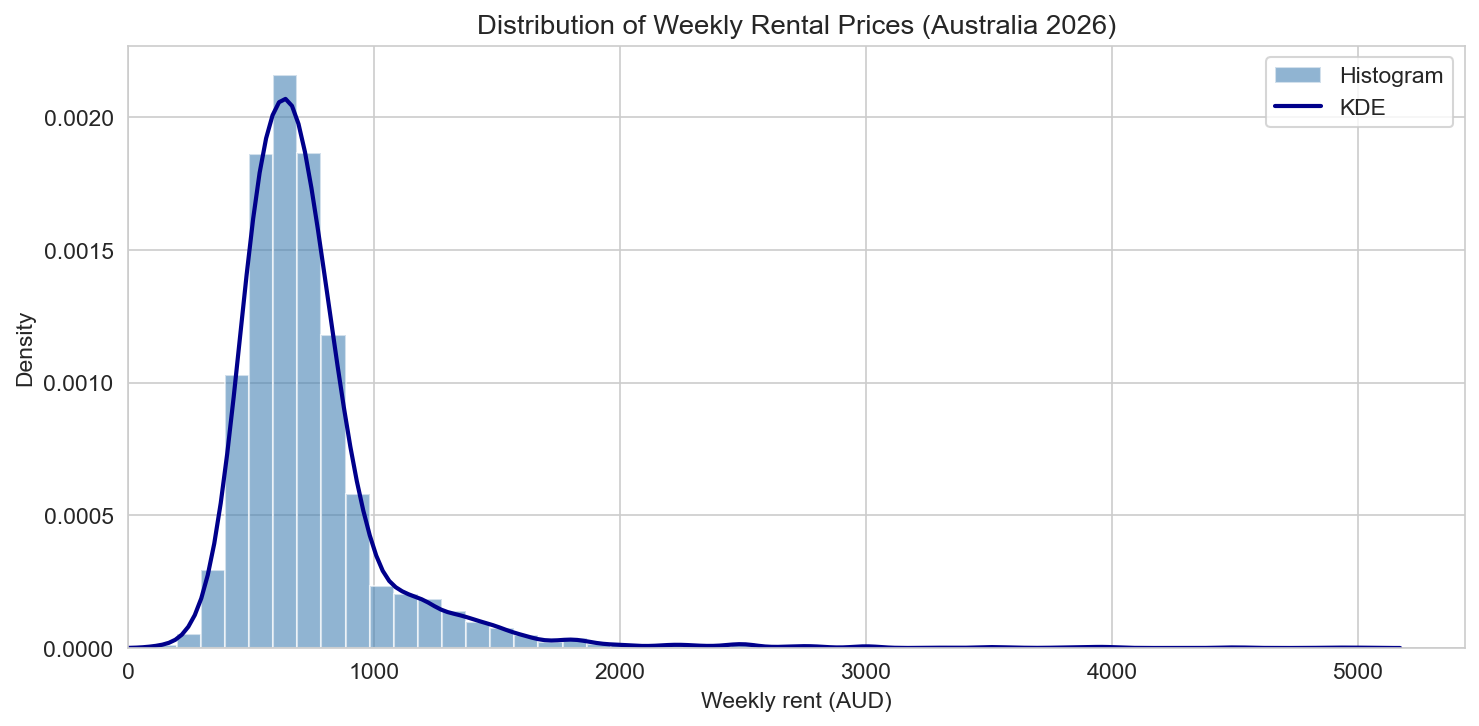
In the cleaned sample, median weekly rent is $670 and the mean is about $734. The distribution is right-skewed: many listings sit in the $400–$800 band, with a long tail of higher-priced properties. All figures in this post use AUD per week.
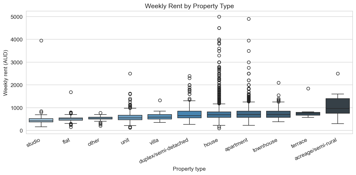
- Property types: Houses, apartments, units, townhouses, studios, and duplex/semi-detached all appear; median rent varies clearly by type, with houses and larger units at the upper end and studios and smaller units at the lower end.
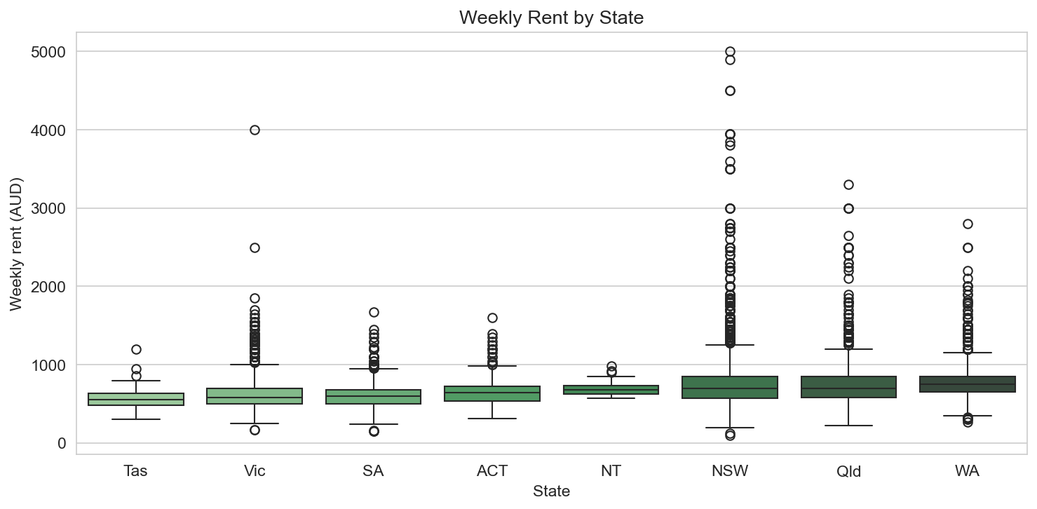
- States: Listings span NSW, Queensland (Qld), Victoria (Vic), WA, SA, and others. Median and mean rent differ by state, reflecting local demand and supply.
- Data cleaning: We dropped rows missing price, coordinates, or bedroom/bathroom counts, and restricted to weekly rent between $100 and $10,000 for a stable analysis sample.
What drives weekly rent (regression)
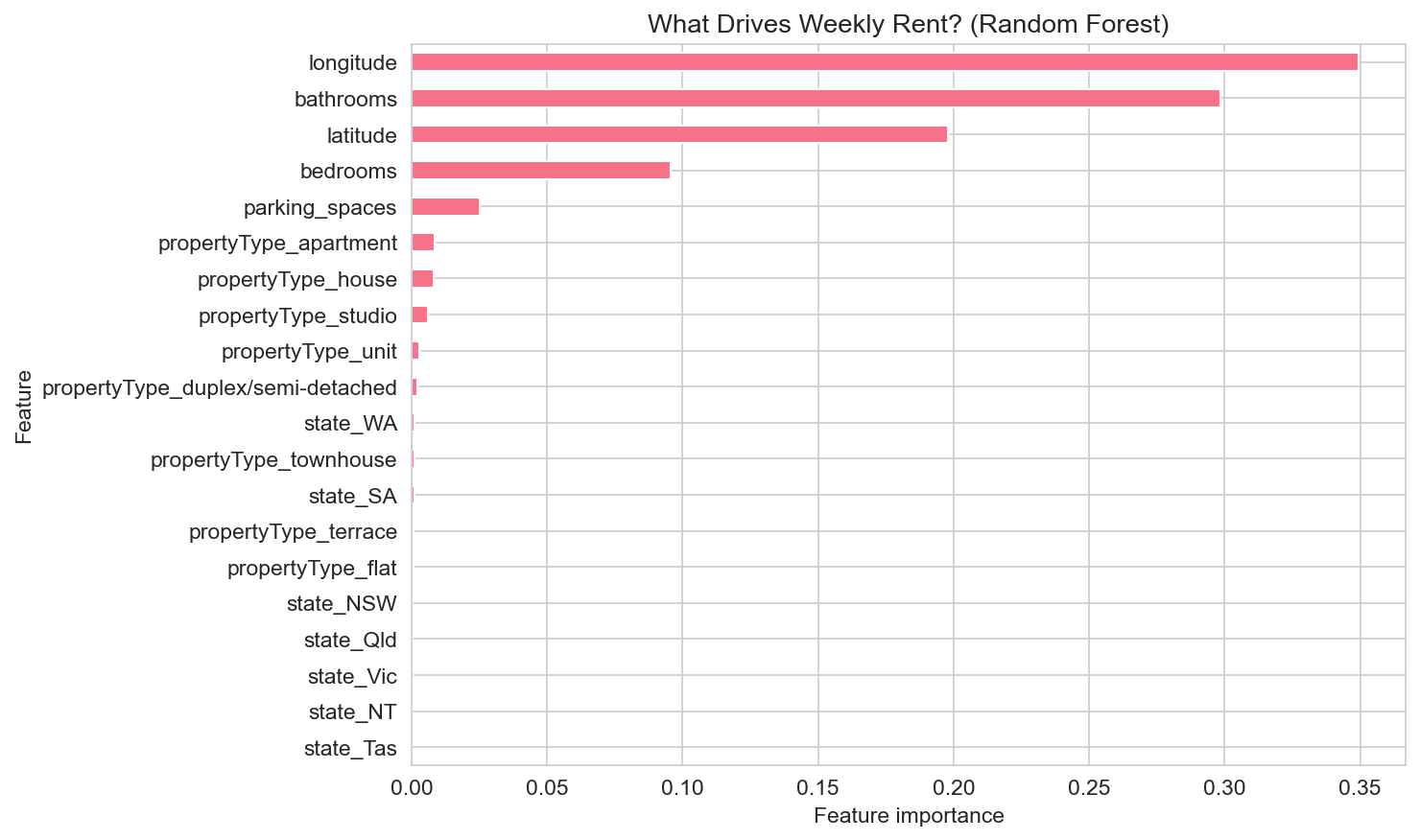
We modeled weekly rent using property and location features: bedrooms, bathrooms, parking spaces, latitude, longitude, property type, and state (one-hot encoded). A Random Forest model explains about 64% of the variance in out-of-sample weekly rent (R² ≈ 0.64), so a meaningful share of rent is predictable from these variables.
Feature importance highlights which variables matter most. Location (latitude and longitude) and bedrooms typically rank among the top drivers, followed by bathrooms, parking_spaces, and then property type and state. So size and location dominate; property type and state add further structure. If you’re benchmarking a listing, start with bedroom count and location, then layer in property type and state.
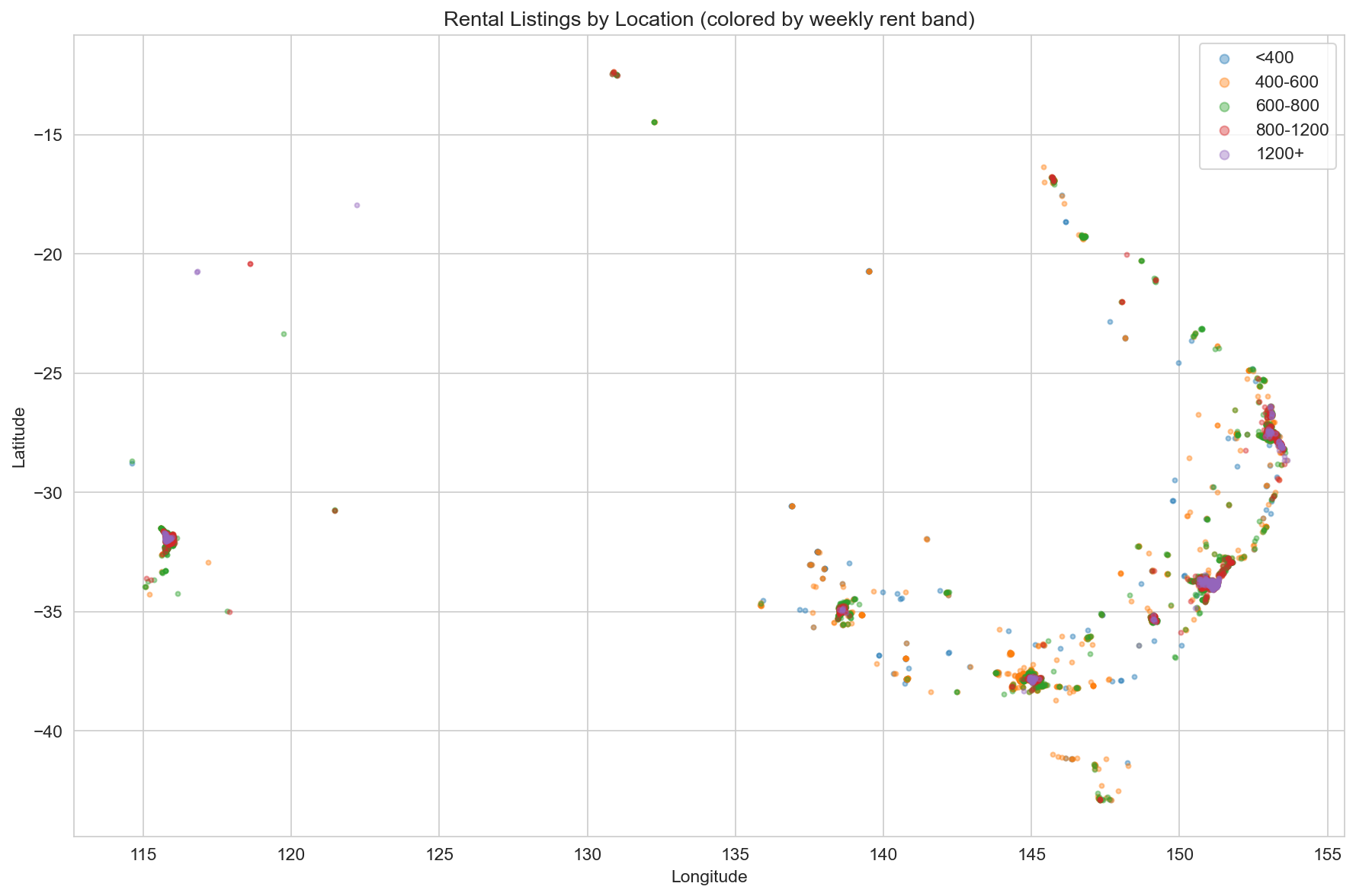
Where rents are highest (geospatial)
Plotting listings by latitude and longitude and coloring points by weekly rent band (under $400, $400–600, $600–800, $800–1200, $1200+) shows clear geographic clustering. Major cities and inner suburbs form high-rent clusters; regional and outer areas tend to fall in lower bands. The map is a simple scatter (no base map), but it makes regional demand hotspots and cheaper corridors easy to see. Renters can use it to compare areas; listers can see how their suburb sits relative to nearby price bands.
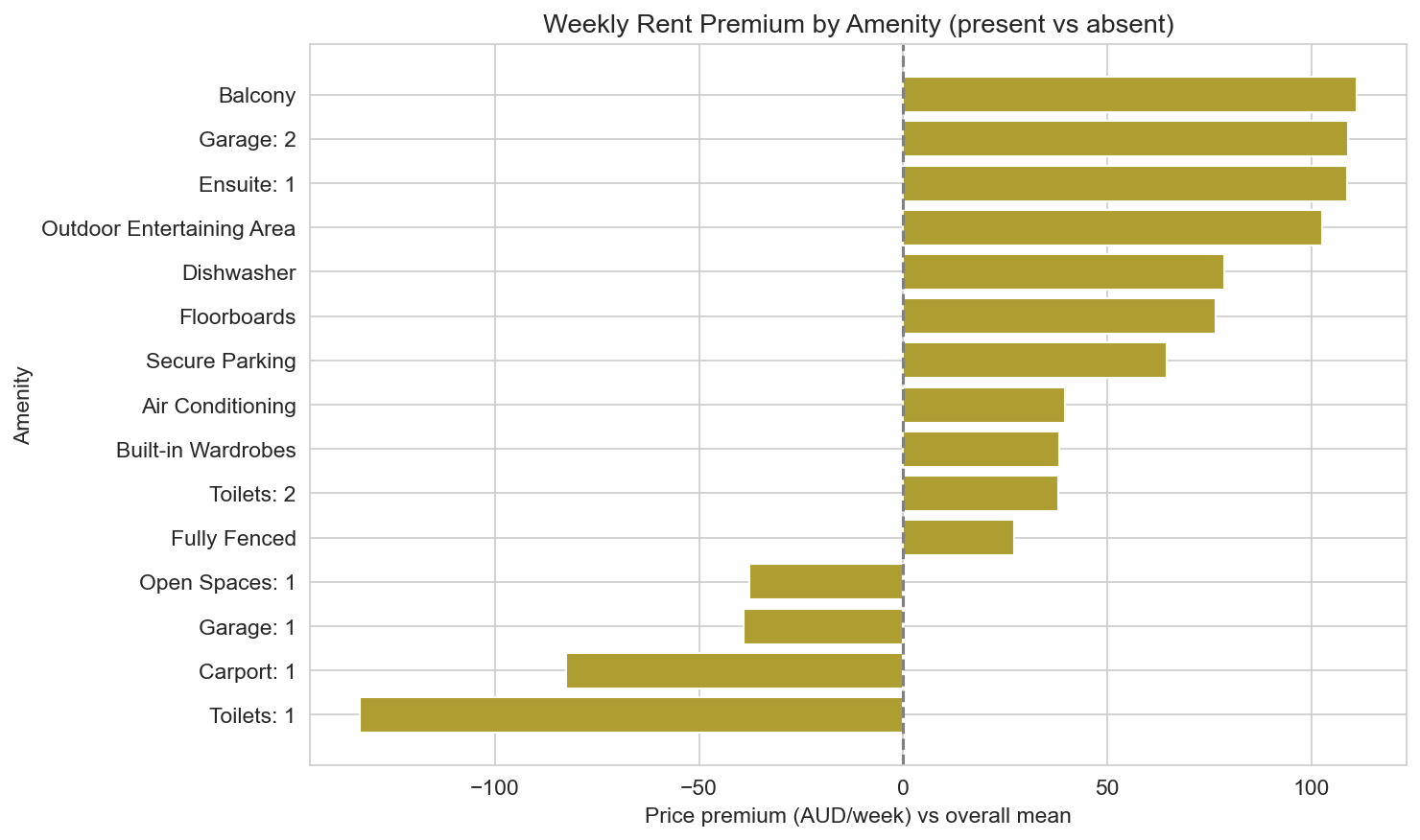
High-value features (NLP and amenities)
We treated amenities as a comma-separated list in each listing and computed the average weekly rent when an amenity is present versus the overall mean. The difference is an “amenity premium” (which can be positive or negative). Some amenities (e.g. certain garage or parking mentions, air conditioning, or lifestyle features) associate with higher mean rent; others appear more in cheaper segments. The chart shows the premium for the most frequent amenities. This is correlation, not causation—listings that mention these amenities may also differ in size and location—but it highlights which features tend to appear in higher-rent listings and can inform how listers describe properties and what renters might prioritise.
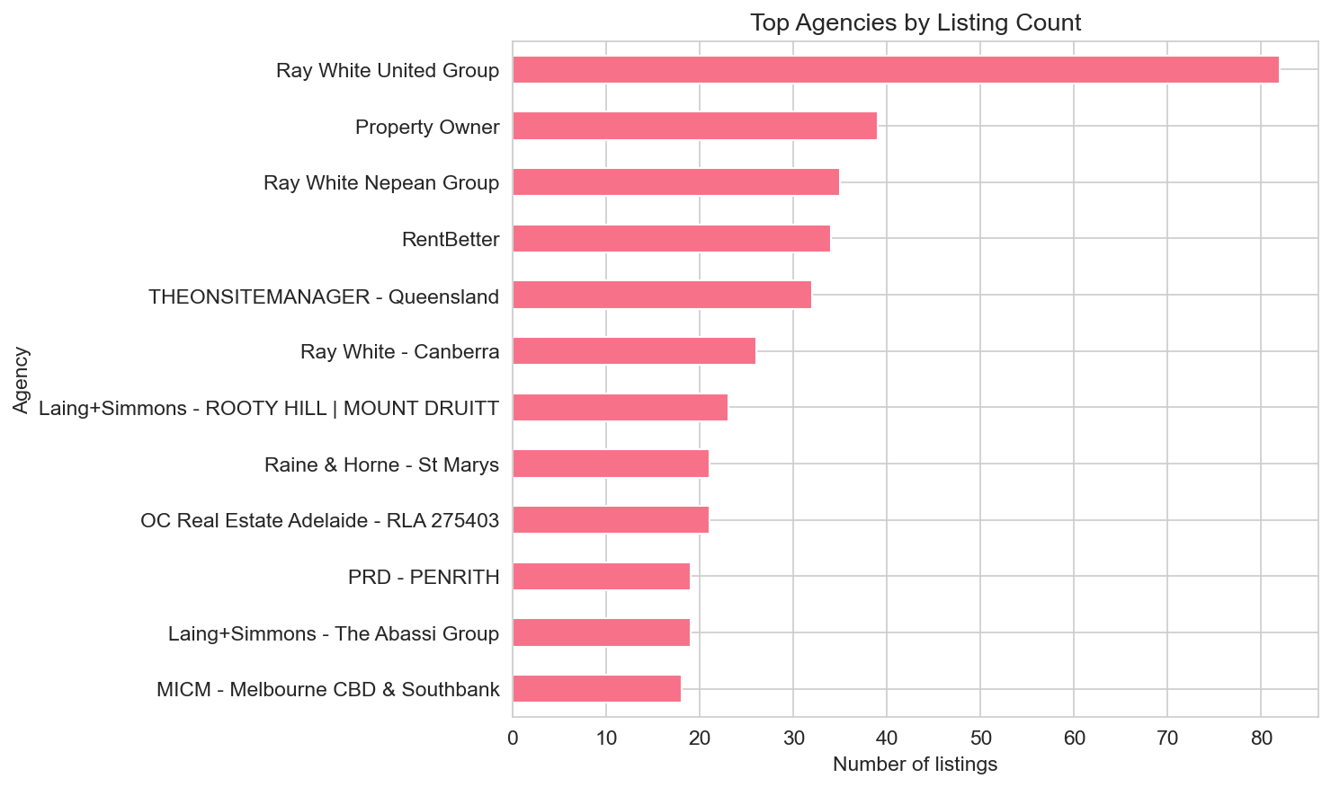
Market segmentation
Agencies vary widely in listing volume. A small set of agencies accounts for a large share of listings; the bar chart shows the top agencies by number of listings. That reflects concentration in property management and which brands are most visible in the sample.
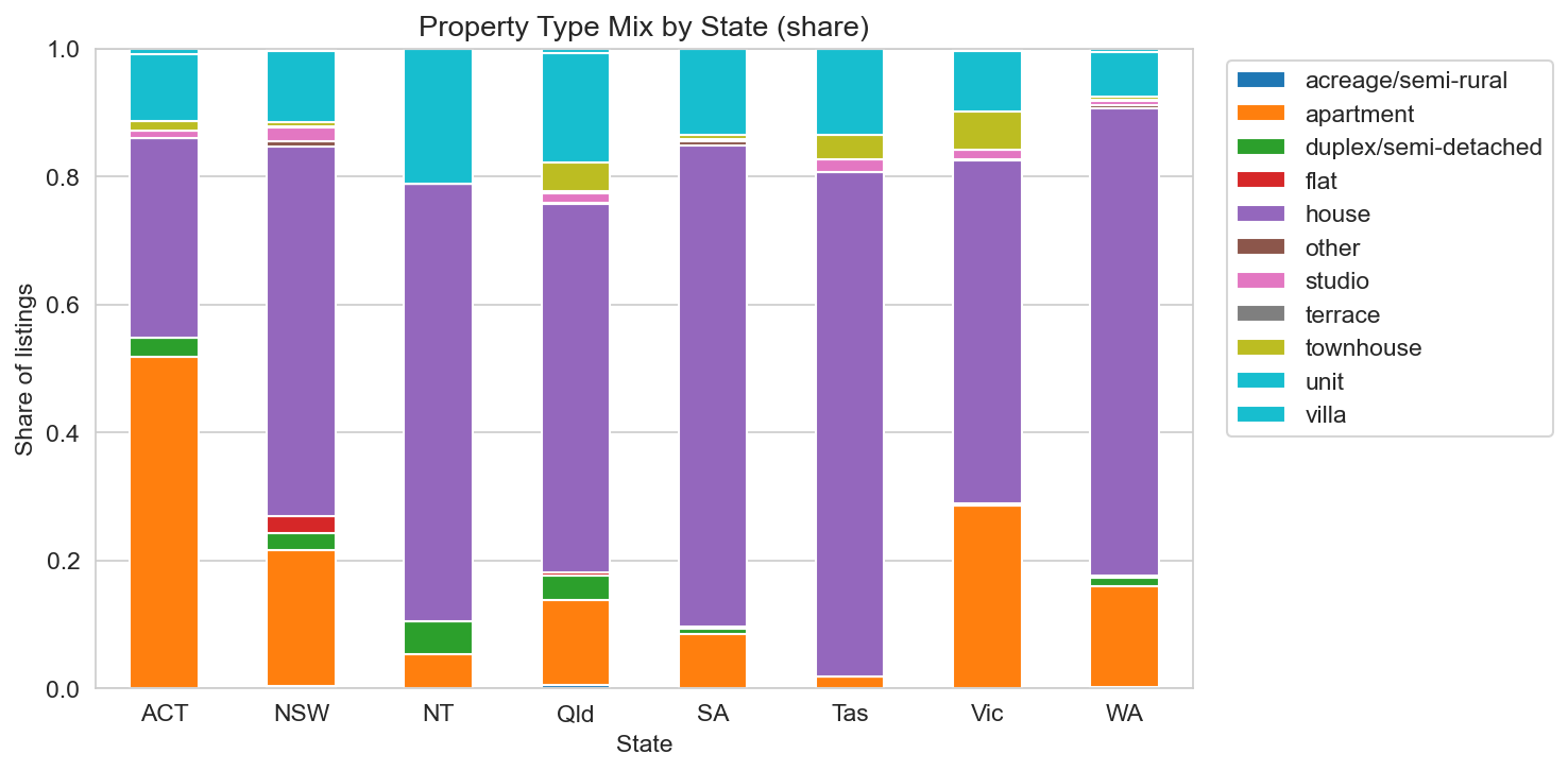
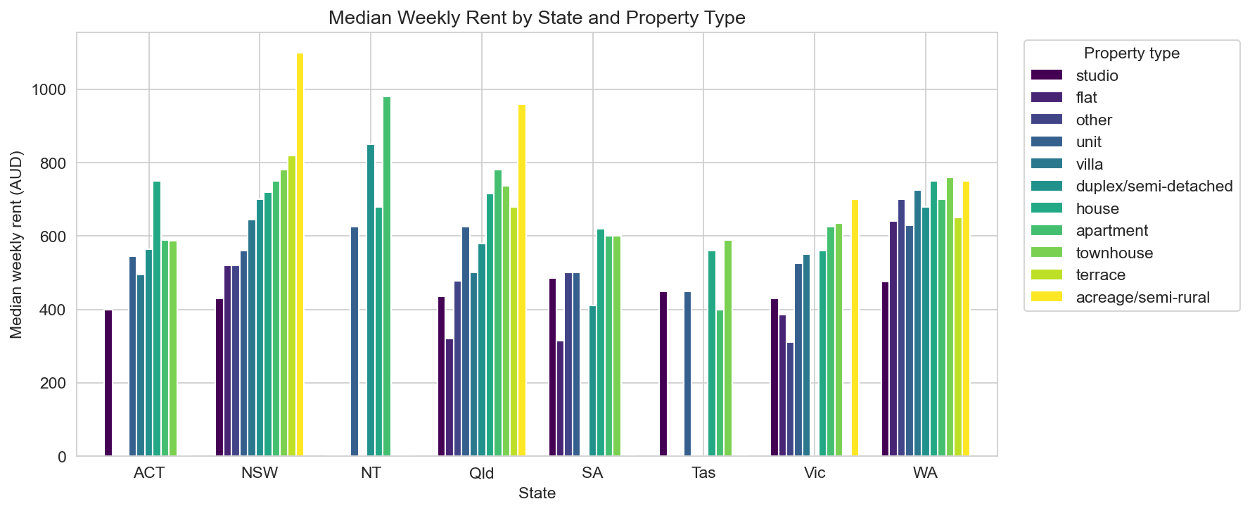
Property type mix by state (stacked bar of shares) shows how the rental stock differs across states: some states have more houses relative to units or apartments. That variation affects median rents and the kind of stock renters can expect in each state.
Median weekly rent by state and property type (grouped bar) summarises the combination of geography and type. Certain state–type pairs sit at the top of the rent distribution; others are more affordable. Together, these views describe the competitive landscape: who lists the most, what type of stock dominates where, and what median rent looks like by segment.
Practical takeaways
For renters
- Use median and mean weekly rent ($670 and ~$734 in this sample) as anchors; then filter by property type and state for your target area.
- Bedrooms and location drive most of the predictable variation in rent; use the geospatial map to see how your preferred areas compare by rent band.
- Amenities that correlate with higher rent in the data may be worth prioritising if you value them; treat the premium chart as a signal of what tends to appear in pricier listings, not a strict price adder.
For listers and agents
- Regression and feature importance show that size and location are the main levers; accurate bedroom/bathroom/parking and location data are central to how rent is set and discovered.
- Market segmentation (agency volume, type mix by state, median rent by segment) helps place your listings in the competitive landscape and set expectations by state and property type.
- Amenity wording that aligns with high-rent segments (e.g. parking, air conditioning, outdoor space) may help listings match tenant search behaviour; keep descriptions accurate and consistent with the data.
Conclusion
The Australian rental sample we analysed shows weekly rents centred around $670 (median) and ~$734 (mean), with clear variation by property type and state. A Random Forest model using property and location features achieves an R² of about 0.64, with location and bedrooms among the strongest drivers. Geospatial plots reveal rent bands and regional hotspots; amenity-level analysis highlights features that tend to appear in higher-rent listings; and segmentation by agency and state illustrates the mix of stock and median rents across the market. Whether you’re renting or listing, using this kind of data can make expectations on price, location, and amenities more concrete.
Data and methodology
The analysis uses the Australian Rental Market Data 2026 dataset (Kaggle: kanchana1990/australian-rental-market-data-2026): listings with title, price_display (weekly rent in AUD), description (HTML), propertyType, locality, latitude, longitude, postcode, state, street_address, suburb, bathrooms, bedrooms, parking_spaces, agency_name, and amenities. Rows with missing price, coordinates, or bedroom/bathroom counts were dropped; weekly rent was restricted to $100–$10,000; parking was imputed when missing. Descriptions were stripped of HTML for potential text analysis; amenities were split on commas for keyword and premium analysis. Regression used scikit-learn (Linear Regression and Random Forest); figures were generated with pandas and seaborn. All results are indicative of the sample and time period; they are not a census of the Australian rental market. Currency is AUD; rent is per week.


